Lab 8 - Spectral Signature Analysis

For this lab exercise we were instructed to collect a number of spectral signatures from a Landsat ETM+ Image.  I did this using the signature editor, digitizing tool and signiture mean plot.  The image I analyzed is displayed below.

I found the following information on the features spectral signitures:
Standing Water:
Highest: band 1(.45-.52), Lowest: band 6(.52-.60)
Reflectance is highest in band one because this is the blue band in the visible spectrum.  After the first three bands, reflectance goes down significantly because there is very little outside of the visible spectrum.

Moving Water: Band 1 (.45-.52) has the highest reflectance

          Band 6 (10.4-4.5) has the lowest reflectance

Vegetation: Band 4 (.77-.90) has the highest reflectance

          Band 6 has the lowest reflectance

Riparian Vegetation: Band 4 has the highest reflectance

          Band 6 has the lowest reflectance

Crops: Band 4 has the highest reflectance

          Band 6 has the lowest reflectance

urban grass: Band 4 has the highest reflectance

          Band 6 has the lowest reflectance

dry soil: Band 5 (1.5-1.75) has the highest reflectance

          Band 4 has the lowest reflectance

moist soil: Band 5 has the highest reflectance

          Band 2 (.52-.60) has the lowest reflectance

rock: Band 5 has the highest reflectance

          Band 4 has the lowest reflectance

asphalt: Band 5 has the highest reflectance

          Band 3 (.63-.69) has the lowest reflectance

airport runway: Band 5 has the highest reflectance

          Band 4 has the lowest reflectance

Concrete: Band 5 has the highest reflectance

          Band 4 has the lowest reflectance

 

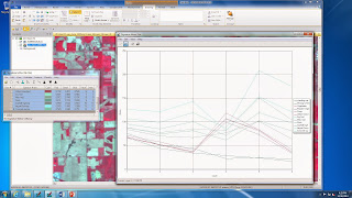
Shown below is a screen shot of all  of the spectral signitures in one graph.

Vegetation displayed high reflectance in band 4, which is the NIR band, and low reflectance in band   The reason that reflectance was so high on the NIR band was because there is a great deal of radiant flux energy reflected at this wavelength and there is a lot of chlorophyll on green vegetation.  In NIR, reflectance is high for green vegetation.

 Band five has the greatest variation between dry and moist soil.  This covers the wavelength range from 1.55 to 1.75 and is the short wave infrared band.  The reason that this wavelength has the most variation is because the shot wave infrared band picks up moisture content very well and can be used to distinguish between moist and dry soil.

Vegetation, crops and grassland are all similar in appearance because they peak at band 4, due to high reflectance in the NIR band.  Standing and moving water are very similar in appearance and have fairly low values across the board and are highest in band one.  Soils are similar but vary in band 5 due to different moisture contents picked up by short wave infrared.  Rock and asphalt are similar in appearance, as well as the runway and concrete.  There seem to be four distinct groups of patterns and each of the four are unlike the others.

It seemed like the most important wavelengths in this exercise were bands 1,4, and 5.  Band one is valuable in identifying elements like water, soil and vegetation.  Band 4 is valuable for analysis on the reflectance of vegetation.  Band 5 is important for analysis of moisture content, especially in soils and vegetation.  I think these are the three most important bands.

 Works Cited:

NASA Landsat Program, 2000, Landsat ETM+ scene, SLC-Off, USGS, Sioux Falls, 2013. 

Lab 7 - Photogrammetry

In this lab exercise we explored photogrammetric tasks on remotely sensed images.  The lab worked with skills in photographic scale, measurement and relief displacement.

For the first part of the lab we calculated scale on a verticle photograph.  Using a ruler, I calculated the scale of the photograph below.

I determined the scale of the photograph was 1:40,000.

. 2.70 in / 8822.47 ft  = 2.70 in / 105869.64 in = 1:39210.98 = 1:40000

 152mm / (20000ft – 796ft) = .50ft / 19235ft = 1:38470 = 1:40000

In the second part of the lab I used the same areal photograph in Erdas Imagine to measure some of the features. First, I calculated the area of the lagoon, then the perimeter, using the digitizing tool in Erdas.

Area = 38.0290 hectares

                   = 93.9716 acres

  Perimeter = 4070.87 meters

                             = 2.5295 miles

I then calculated the relief displacement:

(105.9ft x 10.3 in) / 3980ft = 105.9ft x .86ft / 3980 ft = 0.023 ft

 

In the next part of the lab I used ground control points to show a 3-dimensional perspective of Eau Claire in Erdas Imagine. I did this by generating an anaglyph of the Eau Claire area and found the following results in the output image.

The image clearly represents elevation.  It appears that the darker places in the image represent higher elevation and the lower spots represent higher elevation.  You can tell there are noticeable differences in areas that are different types of land, for example you can see that highly populated areas and areas that are unpopulated seem to stand out somewhat.  The rivers are light in color because they are lower in elevation and the hills are darker in color due to their high elevation.

These features are slightly different from reality.  You can tell that some of the areas like the more heavily populated areas and the heavily vegetated areas seem to have elevations that may not be exactly accurate.  When you zoom in you can tell that there are some specs and areas that do not look natural.  The elevation in higher and more hilly areas seems somewhat exadurated.

Factors that may have caused some difference in the anaglyph could be related to what the anaglyph pick up from the image.  The presence of man-made structures and densely populated areas may have an effect on how the elevation looks.  Also, the amount of ground cover could have an effect.  There is also a large difference in the spatial resolution between the input image and the DEM.  We also increased the vertical exaggeration before making the anaglyph.

In the next part of the lab I orthorectified an image in Erdas Imagine with the used of ground control points.  Below is a screen shot of the two orthorectified images I produced.

In terms of the spatial accuracy, the two orthorectified images match up fairly well.  When zoomed out, you can see a dark line separating the two images and they do not appear perfectly seamless, but when you zoom into the middle of the boundary on the images you can see that they fit together fairly well and the locations of the features seem to match up nicely.  The most noticeable difference at the boundaries is the difference in tone between the two images.  Some areas in the overlapped portion of the image appear darker in color, for tones of grey and dark grey, than they do on the ortho_pan.img.  At the bottom of the overlapped image there is a small gap divided by a black line of pixels that looks like it might cause some problems with spatial accuracy, like slight differences in the positions of common features.

Works Cited:

NASA Landsat Program, 2003, Landsat ETM+, SLC-Off, USGS, Sioux Falls, 2013.

Lab 6 - Geometric Correction

In this lab, I explored different types of Geometric correction.  The first task deals with image-to-map rectification, using a USGS survey digital raster graphic image of Metropolitan Chicago to correct a Landsat TM image.  I also preformed map-to-map rectification on a distorted Landsat TM image, using a correctet Landsat TM image. 

In part one of the Lab I was given a distorted image that needed to be rectified using a reference map image.  I used a USGS 7.5 minute digital raster graphic map of the Chicago Metropolitan area, Chicago_drg.img, to correct the distortion on a Landsat TM image, Chicago_2000.img.  I rectified the Landsat TM image using Image-to-map rectification, through the placement of ground control points.

I preformed the image-to-map rectification using a first order polynomial model. This was done using the multipoint correction window in Erdas Imagine.  Below is a screan shot of the multipoint correction window with all of the GCPs placed on the distorted image and the reference image.  I was able to get the RMS error down below 2.0 to ensure that the correction was done properly.

The Chicago_drg.img serves as a reference map for preforming image-to-map rectification geometrically correcting the Chicago_2000.img to produce a planimetric image.  Ground control points were placed on both images in the same geographic positions in order to preform spatial interpolation, which uses the GCPs to rectify the pixel placement in the output image.  Chicago_drg.img is a digital raster graphic, which is a scanned topographic map used as a reference to the Landsat image Chicago_2000.img.The resampling dialog window is preforming spatial interpolation, which means it is using the ground control points found on both images to perform a geometric coordinate transformation used to rectify pixel location in the output image with the input image.  The resampling method is nearest neighbor.   The four points are spread across the image in order to make an accurate geometric correction.  The distortion in the image is not only in one specific area, it is spread throughout, so the ground control points need to be spread apart.    The first order polynomial model is used in this geometric correction because there were 4 ground control points collected.  A second order of transformation would require a minimum of 6 ground control points and a first order polynomial only requires 3. The minimum number of ground control points needed to perform a 1^st order polynomial transformation is 3.

In the second part of the lab I preformed image-to-image rectification.  I was given a distorted image of Sierra Leone, sierra_leone_east1991.img, and a correct Landsat TM image, sierra_leone_east1991grf.img, to use to geometrically correct the distorted image.  I used a third order polynomial to rectify the distorted image.  Below is a screen shot of the of the Multipoint geometric correction window showing the 12 GCPs that I placed throughout the image. I was able to get the RMS error below 1.0 to ensure proper correction.

   This reference image is in a horizontal coordinate system.  The projection is UTM (zone 29) and the datum is WGS 84. The minimum number of ground control points needed to perform a 3^rd order polynomial transformation.  The polynomial order was set to three in the polynomial model properties and the minimum ground control points needed to perform a third order polynomial transformation is 10, so this minimum must be reached in order for the model solution to be current.  Part one had a first order polynomial transformation, so it only required a minimum of 3 points.   The rectified image is far more geometrically correct compared to the reference image.  It is very apparent that there is much less distortion in the rectified image.  In this correction I used bilinear interpolation instead of nearest neighbor, which is the default setting. Bilinear interpolation is more spatially accurate than nearest neighbor and the output image appears smoother because bilinear interpolation uses the brightness values of the four closest pixels to calculate an output pixel and nearest neighbor only uses the brightness value of the closest input pixel.

Works Cited

 NASA Landsat Program, 2000, Landsat TM scene Chicago_2000.img, SLC-Off, USGS, Sioux Falls, 2000.

NASA Landsat Program, 1991, Landsat TM scene sierra_leone_east1991.img, SLC-Off, USGS, Sioux Falls, 2000.


NASA Landsat Program, 1991, Landsat TM scene Sierra_leone_east1991grf.img, SLC-Off, USGS, Sioux Falls, 2000.

 United States Geological Survey, 2000, digital raster graphic scene Chicago_drg.img, SLC-Off, USGS, Sioux Falls, 2000.

 

Remote Sensing Lab 5

In this lab I have been introduced to a number of skills that take multiple images and put them together to create one seamless image.  In Erdas Imagine, I have used the following tools: RGB to IHS transform,  IHS to RGB transform, Image mosaic, spacial image enhancement, spectral image enhancement, band ratio, and binary change detection. 

In the first part of the lab I have explored color theory and how to transform an image from RGB (Red,Green,Blue) to IHS (Intensity,Hue,Saturation) and back.  I began with a regular RGB image that appeared similar to one you would see in real life colors and transformed it into an IHS image. Below, on the left is the original image and on the right is the newly transformed IHS image.

The new IHS image has totally different colors.  The regular RGB image has similar to real life colors, whereas the IHS image has only tones of red and green.  In the histogram, band one covers a larger brightness area in the IHS image, band two in the IHS image has a brightness concentration towards the edges but is overall low frequencies and is worse contrast than the RGB image.  Band three has a larger range of brightness in the original image but the IHS image has more large spikes in frequency.  Overall, the original image has a more uniform histogram distribution.

Next,  I transformed the IHS image back to RGB and observed the differences between the new RGB image and the original RGB image.   In the histogram, the new RGB image has a wider brightness distribution or higher contrast in Band one.  The histogram appears almost identical for band two.  For band three, the histogram for the original image appears much wider at the base, but the new RGB image has higher frequencies in a more concentrated brightness range.  The colors in the two images appear very similar, but there are some slight differences in tone.  The band combinations are also different.  The original image has a 3,2,1 combination and the new re transformed image has a 1,2,3 combination.

I then repeated the IHS to RGB transformation,  but this time used the stretch I&S tool and then compared the newly stretched RGB image to both the non-stretched and origional RGB images.  Below is a picture of the newly stretched RGB images.

When you switch the color gun to 3,2,1 on the stretched and non-stretched images they turn to a brown and tan tone, while the original image has more of a real looking color range.  You can tell there is differences in the spectral resolution between the three images and the histograms reflect that.  The stretched image is a bit easier to interpret and identify elements when zoomed in.

In the second part of the lab I preformed an image mosaic.  This is preformed by bringing multiple, adjacent satellite images into one seamless image.  I first preformed the image mosaic using mosaic express to produce the image below.

The colors in the output image do not have a smooth transition between the two input images.  There is a very clear boundary between one image and the next.  Both images have mostly tones of black, grey and red, but they are clearly different.  The images have different radiometric properties so they do not appear as one seamless image.

Next, I made another mosaic of the two images but this time using Mosaic Pro using the histogram matching tool.  Then I compared the mosaic images using mosaic pro and mosaic express.  Below is a screenshot of the image created using Mosaic Pro.

 

   The output image using MosaicPro is a much more seamless image than the Mosaic Express image.  The MosaicPro images blend into each other much better and the tones are similar between the two images.  The tones are similar in the Mosaic Pro image because of the histogram matching color correction function.  The Mosaic Express image does not appear as seamless because the input images have different radiometric properties and therefor do not blend together well.

In the third part of the lab I preformed band ratioing using the normalized difference vegetation Index.  I then analyzed the colors in the image using NDVI and found the following.

  I would expect that the very white areas would be areas with the most vegetation.  If you zoom into the image, you can tell that roads, rivers and buildings appear darker, while other areas like fields appear very white in color because of the presence of vegetation.   The areas that appear medium grey likely have very little vegetation and the areas that are black likely have almost no vegetation.  The rivers and lakes appear black in the image because no vegetation is detected.  Many of the medium grey spots in the image are more densely populated areas, so they would have less vegetation.

In the fourth part of the lab I explored spatial and spectral enhancement techniques.  First I used spatial enhancement,  specifically high and low pass filters to change images frequency.  A high frequency image is an image that has large changes or variance in brightness values over short distances.  A high frequency image may need to be suppressed using spatial filtering to improve the spatial frequency.    A low frequency image has small differences in brightness over larger distances.  The image may appear hazy and not clear or defined, requiring filtering in order to improve the spatial frequency.

First I used a 5x5 low pass filter and compared the output image with the origional image.  The original image is more clear and defined than the 5x5 low pass filtered image.  When you zoom in on the two images, you can see more detail and it is easier to interpret the original image.  The low pass filter image has a lowered spatial frequency, so it has smaller changes in brightness over areas in the image.

Then I preformed a 5x5 high pass filter and compared the output image to the origional image.   The high pass filtered image is much more defined and clear than the original image.  The high pass filtered image uses a black tone to replace a lighter grey tone in the original image. When you zoom in to the images, the original appears cloudier and less defined due to the lower frequency.  The high pass filtered image is easier to interpret and has more contrast.

Next,  I worked with edge enhancement, using a laplacian convolution filter.    A laplacian convolution filter is a linear edge enhancement tool used to delineate edges in an image in order to make elements of an image more clear and easy to interpret.  It calculates a new derivative between pixels which creates a higher contrast in order to make an enhanced image.  I took an image and applied the laplacian convolution filter.  The original image appears much different than the laplacian edge detection image.  When zoomed out, the original image has tones of mostly green at the top and red at the bottom, whereas the laplacian edge detection image appears darker in color, with mostly tones of green and purple and a cloudy checkered look.  When zoomed in, the laplacian edge detection image is darker in color but has brightly colored blue and green specs and red lines.  The original image is mostly a mix of red and green features that are easier to differentiate between.

In the next section,  I worked with spectral enhancement, preforming two types of linear contrast stretches.  First I used a minimum-maximum contrast stretch because this is a low contrast histogram, with a high frequency in a very small brightness range.  It is somewhat uniform or gausian.  One peak or mode.   It is appropriate to use a min-max contrast stretch because the input image has a low contrast, with a high frequency in a very small brightness range and a min-max contrast stretch can be used to expand the brightness range, giving the image a higher contrast. The histogram will become much wider and cover more brightness values.  Min-max contrast stretch is appropriate for gausian or near gausian histograms.  Below is a screen shot of the contrast stretch.

I then preformed a piecewise contrast stretch on a different image.  This image
Histogram has multiple peaks that represent modes.  It is not perfectly gausian and it has a higher contrast that covers the lower end of the brightness values.  A piecewise contrast stretch is necessary because it can expand the brightness ranges of multiple modes or peaks.  Because the histogram is not gausian, piecewise stretch is appropriate.  Below is a screen shot of the piecwise contrast image.

 

I then compared the piecewise contrasted image with the origional input image.   The piecewise contrast stretched image is definitely more clear and easy to look at.  It really brought out the medium grey tones so they stand out more from the light grey tones and you can tell the black became much darker and solid.  The piecewise contrast stretched image is definitely easier to interpret.

In the next section I used Histogram equilization to improve the contrast of an image.  The origional image histogram has one mode and is fairly gausian.  It is low contrast and hits a very small brightness range.  The image looks to be a little hazy and white in color in the more urban areas and darker everywhere else. The histogram equalized image has a better range of color and brings out the details much more than the original image.  You can see vegetation very well in the histogram equalized image.  The histogram for the new image appears totally different, it is completely filled in the bottom of the brightness range and then has steps going up and down at right angles.  The brightness range also starts at 39 instead of 0 on the histogram.

In the fifth part of the lab I used Binary change detection and image differencing to estimate brightnessvalues of pixels between two images of Eau Claire,  one taken in 1991 and the other taken in 2011.  I used the histogram of the differenced image to find the upper limit of change-no change threshhold and the lower end change-no change threshold.  I also found the upper and lower limits using this histogram:

 

Finally,  I used model maker to model the change between the two images.  This is what I found regarding the spatial distribution of areas changed over the 20 year perioud:

  It looks like you see the most change in urban centers, but you do see specs of change spread throughout.  You see the most change along the river and in the northwest corner of the image. There are definitely patches that have large amounts of change that appear darker.  There are dark patches surrounding the Eau Claire city center and around the Chippewa Falls area.

Works Cited

 NASA Landsat Program, 1991 - 2011, Landsat ETM+, SLC-Off, USGS, Sioux Falls, 11/11/13.


































 

Remote Sensing Lab 4 - Image Functions

            The goal of this lab is to demonstrate how to enhance images in order to preform analysis and also to focus in on a precise area in a large satellite image.  I have delineated the area of interest from a large image, explored techniques to enhance spatial and radiometric resolution, linked Google earth with Erdas Imagine, and used bilinear and nearest neighbor resampling methods. 

            The first part of the lab deals with subsetting images using an inquire box and an area of interest shape file.  First I made an image subset of the Eau Claire area using an inquire box found in the raster tools. 

Next, I used a shapefile to create an area of interest file.  This was done using the subset and chip option in the Raster tools.         

            In the second part of the lab exercise, I have used image fusion to improve the spatial resolution of an image.  I did this using the resolution merge icon in the pan sharpen tools.  First I used the nearest neighbor resampling technique.

 

Then I used the bilinear interpolation resampling technique to fuse the images. 

Both strategies of image fusion result in a pan sharpened image.  The pan sharpened image definitely has a greater range of colors, brighter colors and a higher resolution than the input image.  A pan sharpened image has a higher spatial resolution, which is noticeable especially when you zoom in on the images.  The pan sharpened image also has a larger range of more vibrant tones, the river is a darker black and the pinks are slightly darker or bolder.  Much of the area that was a light blue tone in the input image is more of a grey in the pan sharpened image.

                In part three of the lab I improved the radiometric resolution of an image using the haze reduction tool under radiometric in the raster tools.  The input image is much lighter in color and cloudier than the haze reduction image.  When you zoom in and out the resolution of the images is the same but the colors are definitely brighter and clearer in the haze reduced image.  There are a few places in the input image that have light colored clouds or haze and these do not appear in the haze reduced image.  The rivers went from a blue color to black and the pinks went to more vibrant red tones.  The haze reduced image is definitely clearer.

 

                In part four of the lab I have linked Google Earth with Erdas Imagine in order to create synchronized views of an image.  This was done using the connect to google earth icon, then selecting match GE to view and Link GE to view icons. You can zoom in very close at a high resolution on the google earth viewer, which can be very useful if you are trying to identify elements of an image.  When you zoom in it becomes much easier to identify objects on the google earth image and there are some labels.

                In part five of the lab I used resampling to change the pixel size of an image.  This was done by selecting resample pixel size under spatial in the Raster tools tab.  I changed the output cell size to 20 meters, from the input cell size of 30 meters. I used the nearest neighbor method for the first output image, then the bilinear interpolation method for the second.

 

 There is some difference in the pixilation between the input image and the nearest neighbor resampled image.  When you zoom in very close, you can notice that the pixel size is smaller in the nearest neighbor image and that the formation of the pixels is slightly different.  When zoomed out very far it is hard to tell the difference between the images.  The nearest neighbor method uses the brightness and tone of the closest pixel. The bilinear interpolation image is also similar to the original image when zoomed out, but definitely has a different pixel formation when closely zoomed in.  The bilinear interpolation uses the tone and brightness that is calculated using the four surrounding pixels.  This results in a pixel formation different from the original image and the nearest neighbor image.

Works Cited

"Earth." Google. N.p., n.d. Web. 01 Nov. 2013

 "Welcome to the USGS - U.S. Geological Survey." Welcome to the USGS - U.S. Geological Survey. N.p., n.d. Web. 01 Nov. 2013